Our behaviour is often very variable and reducing it to single number such as an average might be comforting but ultimately misleading. For instance, I generally use 500MB of data on my cellphone on a monthly basis but this can be as little as 200 MB and on occasion well beyond 1GB. This line of thinking would suggest my behaviour is best modelled as a distribution with a peak around 500MB and a mean just above 500MB. Latent Class Analysis attempts to recover these distributions of behaviour for groups of customers.
I am going to simulate a cellphone dataset where the segments represent different distributions of cellphone usage. The advantage of simulation is that we know the true process that the data was generated so we can check if the model gets the answer right. Simulation also allows us to test how sensitive our model is to sample size (will not cover this though) and it removes the gremlins/detail of real data which often take up 80% of the time to resolve/understand.
The Figure 1 below shows the 5 segments hidden in the data we will simulate:
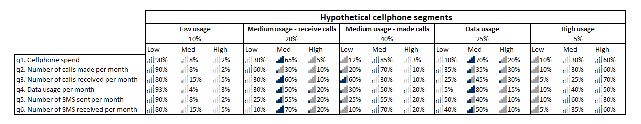
From the Figure 1, you should see that 10% of customers fall into the ‘low usage’ segment. Our segmentation base consists of 6 variables. All variables have 3 levels denoting intensity of usage - Low, Medium, High. A ‘low usage’ customer is expected to have a ‘Low’ cellphone spend 90% of the time, ‘Medium’ spend 8% of the time and ‘High’ spend 2% of the time. It is important to note the segments have overlapping distributions which makes deciding the distribution a customer belongs to difficult a exercise.
The analysis below was implemented using R. Snippets of code have been included for those familiar with the language to give a more concrete understanding.
set.seed(201603)
no.of.cust <- sample(1:5,5000,replace=TRUE,prob=c(0.1,0.2,0.4,0.25,0.05))
I have set the the seed to ensure the numbers are reproducible but this is not entirely necessary. We generate a sample of 5000 cellphone customers with 10% in ‘low usage’, 20% in ‘medium usage - receive calls’, etc.
sz.of.seg <- table(no.of.cust)
sz.of.seg
## no.of.cust
## 1 2 3 4 5
## 498 1010 2003 1268 221We tabulate our customer sample into a table of counts.
#probability matrix for 'low usage' segment
low.usage <- matrix(c(0.9,0.08,0.02,             #distribution on q1
		      0.9,0.08,0.02,             #distribution on q2
		      0.8,0.15,0.05,             #distribution on q3
		      0.93,0.04,0.03,            #distribution on q4
		      0.9,0.08,0.02,             #distribution on q5
		      0.8,0.15,0.05),            #distribution on q6
		      nrow=6,ncol=3, byrow=TRUE)

#probability matrix for 'medium usage - receive calls' segment
med.usage.rec.calls <- matrix(c(0.3,0.65,0.05,   #distribution on q1
				0.6,0.3,0.1,     #distribution on q2
				0.3,0.6,0.1,     #distribution on q3
				0.3,0.5,0.2,     #distribution on q4
				0.25,0.55,0.2,   #distribution on q5
				0.1,0.7,0.2),    #distribution on q6
				nrow=6,ncol=3, byrow=TRUE)

#probability matrix for 'medium usage - made calls' segment
med.usage.made.calls <- matrix(c(0.12,0.85,0.03, #distribution on q1
				 0.2,0.7,0.1,    #distribution on q2
				 0.6,0.3,0.1,    #distribution on q3
				 0.3,0.5,0.2,    #distribution on q4
				 0.25,0.55,0.2,  #distribution on q5
				 0.1,0.7,0.2),   #distribution on q6
				 nrow=6,ncol=3, byrow=TRUE)

#probability matrix for 'data usage' segment
data.usage <- matrix(c(0.1,0.7,0.2,              #distribution on q1
		       0.35,0.35,0.3,            #distribution on q2
                       0.25,0.45,0.2,            #distribution on q3
                       0.05,0.8,0.15,            #distribution on q4
                       0.5,0.4,0.1,              #distribution on q5
                       0.4,0.5,0.1),             #distribution on q6
		       nrow=6,ncol=3, byrow=TRUE)

#probability matrix for 'high usage' segment
high.usage <- matrix(c(0.1,0.3,0.6,              #distribution on q1
		       0.1,0.3,0.6,              #distribution on q2
		       0.05,0.25,0.7,            #distribution on q3
                       0.1,0.4,0.5,              #distribution on q4
                       0.1,0.6,0.3,              #distribution on q5
                       0.05,0.35,0.6),           #distribution on q6
		       nrow=6,ncol=3,byrow=TRUE)
In this section, we translate the distribution tables in Figure 1 into probability matrices for each segment.
cust.data <- rbind(     #combine each simulation result for each segment
			cbind(
				#simulate behaviour for 'low usage' segment
				sample(1:3,sz.of.seg[1],replace=TRUE,low.usage[1,]), #q1
				sample(1:3,sz.of.seg[1],replace=TRUE,low.usage[2,]), #q2
				sample(1:3,sz.of.seg[1],replace=TRUE,low.usage[3,]), #q3
				sample(1:3,sz.of.seg[1],replace=TRUE,low.usage[4,]), #q4
				sample(1:3,sz.of.seg[1],replace=TRUE,low.usage[5,]), #q5
				sample(1:3,sz.of.seg[1],replace=TRUE,low.usage[6,]) #q6
			),
			cbind(
				#simulate behaviour for 'medium usage - receive calls' segment
				sample(1:3,sz.of.seg[2],replace=TRUE,med.usage.rec.calls[1,]), #q1
				sample(1:3,sz.of.seg[2],replace=TRUE,med.usage.rec.calls[2,]), #q2
				sample(1:3,sz.of.seg[2],replace=TRUE,med.usage.rec.calls[3,]), #q3
				sample(1:3,sz.of.seg[2],replace=TRUE,med.usage.rec.calls[4,]), #q4
				sample(1:3,sz.of.seg[2],replace=TRUE,med.usage.rec.calls[5,]), #q5
				sample(1:3,sz.of.seg[2],replace=TRUE,med.usage.rec.calls[6,]) #q6
			),
			cbind(
				#simulate behaviour for 'medium usage - made calls' segment
				sample(1:3,sz.of.seg[3],replace=TRUE,med.usage.made.calls[1,]), #q1
				sample(1:3,sz.of.seg[3],replace=TRUE,med.usage.made.calls[2,]), #q2
				sample(1:3,sz.of.seg[3],replace=TRUE,med.usage.made.calls[3,]), #q3
				sample(1:3,sz.of.seg[3],replace=TRUE,med.usage.made.calls[4,]), #q4
				sample(1:3,sz.of.seg[3],replace=TRUE,med.usage.made.calls[5,]), #q5
				sample(1:3,sz.of.seg[3],replace=TRUE,med.usage.made.calls[6,]) #q6
			),
			cbind(
				#simulate behaviour for 'data usage' segment
				sample(1:3,sz.of.seg[4],replace=TRUE,data.usage[1,]), #q1
				sample(1:3,sz.of.seg[4],replace=TRUE,data.usage[2,]), #q2
				sample(1:3,sz.of.seg[4],replace=TRUE,data.usage[3,]), #q3
				sample(1:3,sz.of.seg[4],replace=TRUE,data.usage[4,]), #q4
				sample(1:3,sz.of.seg[4],replace=TRUE,data.usage[5,]), #q5
				sample(1:3,sz.of.seg[4],replace=TRUE,data.usage[6,]) #q6
			),
			cbind(
				#simulate behaviour for 'high usage' segment
				sample(1:3,sz.of.seg[5],replace=TRUE,high.usage[1,]), #q1
				sample(1:3,sz.of.seg[5],replace=TRUE,high.usage[2,]), #q2
				sample(1:3,sz.of.seg[5],replace=TRUE,high.usage[3,]), #q3
				sample(1:3,sz.of.seg[5],replace=TRUE,high.usage[4,]), #q4
				sample(1:3,sz.of.seg[5],replace=TRUE,high.usage[5,]), #q5
				sample(1:3,sz.of.seg[5],replace=TRUE,high.usage[6,]) #q6
			)
)
The above code creates our simulated data set. To simplify the simulation each question is simulated under conditions of independence. Non-independence simulation is possible but we would have to specify every conditional distribution, that is 4379 parameters rather than 95.
cust.data <- as.data.frame(cust.data)
colnames(cust.data) <- c("q1","q2","q3","q4","q5","q6")
head(cust.data)
## q1 q2 q3 q4 q5 q6
## 1 1 1 1 1 1 1
## 2 1 2 1 1 1 2
## 3 1 1 1 1 1 1
## 4 1 1 1 1 1 1
## 5 1 1 2 1 1 1
## 6 1 1 1 1 1 1A bit of housekeeping, converting the customer data into a dataframe and adding labels.
require(poLCA)
LCA.model <- poLCA(cbind(q1,q2,q3,q4,q5,q6) ~ 1,cust.data,nclass=5,nrep=10,maxiter=100000)
We finally run our latent class model for 5 segments using the polytomous variable Latent Class Analysis package (poLCA). We repeat the run 10 times to ensure we are converging to a global solution rather than a local one. The default iterations are not enough for convergence so I have increased this to 100 000 to reach convergence.
So did poLCA recover our segments?
Well, it is a bit of a mixed bag.
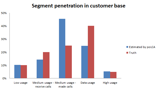 The estimation of the size of the segments with least overlap is within 1% of the truth - ‘Low usage’ and ‘High usage’ segments. It under estimates the size of the ‘data usage’ segment by 15% and over estimates the ‘medium usage - made calls’ segment by 20%.
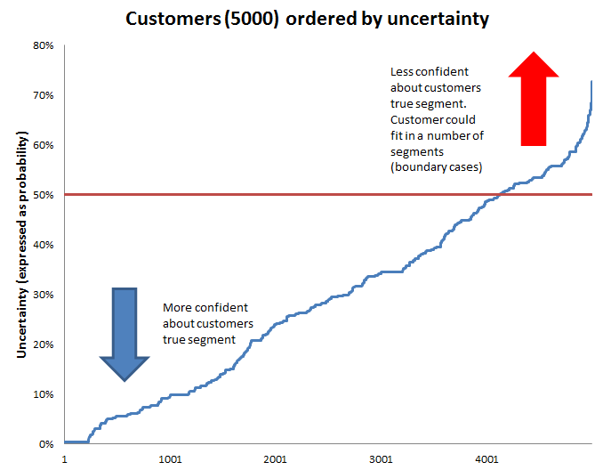 The uncertainty plot indicates that for about 17% (800) of customers it was less 50% confident that the customer belonged in the segment with the highest probability of membership. This helps explain why the penetration estimates were so off.
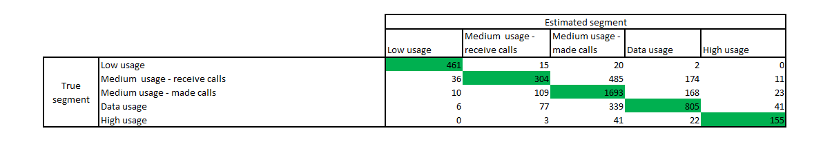 Thanks to simulation we can estimate whether Latent Class Analysis classified the customer in the right segment. poLCA had a 68% accuracy rate looking at the confusion table above. Random guessing would be 20% accurate and classifying everyone into the largest segment is 40% accurate. Human intuition would probably get the segments with the least overlap right (15%) and classifying the rest into the largest segment would push accuracy to around 55%.
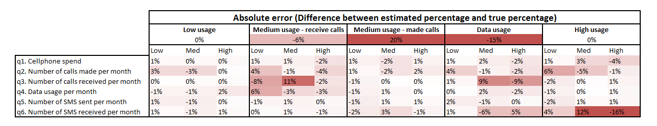 The table shows the accuracy of the model in estimating the 95 parameters for the simulation model. Hopeful it is clear for above summary stats that untangling overlapping behaviours is a tough endeavour. There is a loss of information when moving from the true distribution to the observed behaviour which makes going backwards hard. Latent Class Analysis does at least give us an idea of how uncertain the model is and is possibly the best we can do without being omnipotent.
Final thoughts …
- Should we simplify the problem by merging the ‘data usage’ segment and ‘medium usage - made calls’ segment, this will increase our accuracy but we would become less specific?
- Did not really cover how to determine the best number of segments when you don’t know the true number of segments.
- Will a larger sample size improve matters?
- How do we deal with the stability of the segments especially with growing prevalence of over-the-top content (OTT) in the cellphone industry?
- How do other segmentation algorithms compare such as K-means?